

In this article, we will explore a method to tackle the issue of optimizing inventory management thanks to quantile based time-series predictions and leveraging Atoti — a data visualization platform with an aggregation engine and native multidimensional and what-if analysis support.
Inventory management is one of the most critical components of the manufacturing and supply chain processes. Inventory management is also one of the major issues faced by the industries.
When it comes to sales for the manufacturing industries, both the extreme scenarios are unfavorable:
- When there is an unexpectedly high demand — it will cause stock-outs
- When there is unexpectedly low demand — it will cause dead inventory
The solution: making quantile predictions, and letting the business make decisions
So the solution is to predict the whole spectrum of sales numbers, adjust the inventory or the stocks as per the business risk appetite and hence keep the future demand roughly “as expected.”
The typical mean or median based methods tend to ignore the extreme situations and derive towards the “usual” scenario. Hence, mostly these methods are not very effective at preventing both stock-outs and dead inventory. Quantile based forecasts approach the challenge head-on and directly look at the scenario of interest, say avoiding stock-outs, and strive to provide a precise answer to this very problem.
Advantages of using the quantiles based sales prediction
- Dead Inventory Reduction — One of the significant revenue leakage sources for manufacturing industries is dead inventory, i.e., raw materials that were bought but were never used. The storage of such raw materials is also a cost, so they cannot be stored forever.
- Prioritizing supply chain decisions — The demand forecasts can be used to drive supply chain decisions such as making purchase orders for commerce or triggering a production batch in an industrial setting.
- Injecting the supply chain constraints — There are often constraints by the suppliers for minimum order either at the SKU level or at the order level, and they can be tweaked as per the business desire based on the forecast.
In this article, we will consider the case of a salad manufacturer and perform a sales/demand prediction on a quantile basis and hence giving the business an opportunity to choose how aggressive or reserved they want to be with the inventory acquisition and hence the manufacturing capabilities.
1. Dataset
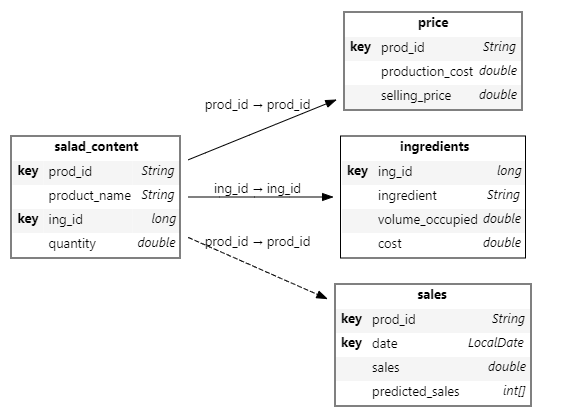
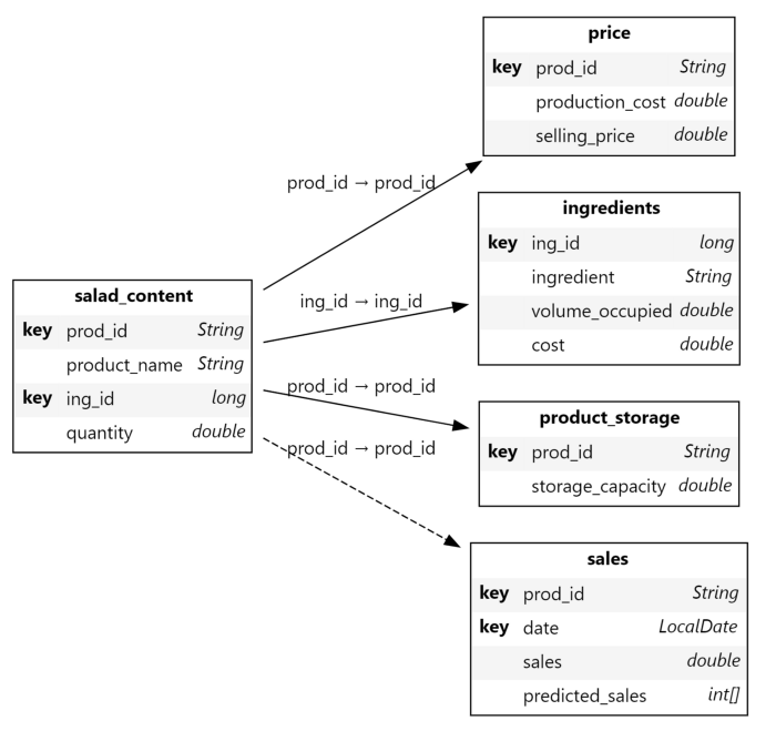
For the various salad products available, we are given the composition of each of them, along with the historical sales values, sales price, and the production cost. Also, we are given the price for each ingredient, the storage volume required to store one kilogram.
Below is a schema of the various datasets available:
Creating the above schema in Atoti is as easy as ABC:
# creating the cube
salad_cube = session.create_cube(salad_content, "SaladCube")
# plotting the schema
salad_cube.schema
2. The sales/demand time-series prediction
Predicting the future has been a long-unconsummated fantasy for the professionals not confined to the manufacturing industries. No matter how fascinating it may seem, trying to predict the “exact-future” using one variable (time-series like predictions) may not only be incorrect but is also somewhat naïve at its basics because no matter how good this variable can be, it can never tell the full story.
In fact, statistical forecasting is very counter-intuitive, and the reality is that there is frequently nothing to fix: the forecasted value is one of the perfectly valid and possible outcomes for future demand.
Hence comes the concept of making quantile based predictions — a phenomenon with the underlying concept that instead of predicting a unique value, let us predict the entire spectrum of values and let the business choose how much aggressive or reserved they want their sales number to be.
Thinking about the future from a completely probabilistic perspective might seem entangling. However, it actually represents what business executives have been doing, though in slightly informal ways: weighing the odds of certain outcomes and hedging the bets vis-à-vis their business in order to be well-prepared when dealing with the most relevant scenarios.
How to do the probabilistic forecasts?
Most traditional time-series predictions predict a single ‘most-likely’ value for the future. Hence, in order to solve this issue, GluonTS is used for making probabilistic forecasts and then the values corresponding to a mist of given quantiles are picked from the forecast.

GluonTS is a python toolkit for probabilistic time series modeling, built around Apache MXNet (incubating). It has been built by the Amazon Web Services — Labs.
GlounTS leverages the truly open-source deep learning framework suited for flexible research prototyping and production at Apache MXNet.
Here is a code snippet to use the GluonTS:
mx.random.seed(36)
np.random.seed(36)

for column in df.columns[1:]:

    training_data = ListDataset([{'start': df.date[0],
                                'target': df[column]}], freq='D')

    estimator = DeepAREstimator(freq='D', prediction_length=60,
                                trainer=Trainer(epochs=1))
    predictor = estimator.train(training_data=training_data)

    test_data = ListDataset([{'start': df.date[0],
                            'target': df[column]}], freq='D')

    for (test_entry, forecast) in zip(test_data,
            predictor.predict(test_data)):
        pass

    globals()['sales_' + str(df[column].name)] = []
    print df[column].name

    for i in np.linspace(0, 0.99, 10):
        globals()['sales_'
                  + str(df[column].name)].append(forecast.quantile(i))

    globals()['sales_' + str(df[column].name)] = \
        np.reshape(globals()['sales_' + str(df[column].name)], (10,
                   60)).T

    globals()['sales_' + str(df[column].name)] = globals()['sales_'
            + str(df[column].name)].tolist()

    print type(globals()['sales_' + str(df[column].name)])

    for (i, item) in enumerate(globals()['sales_'
                               + str(df[column].name)]):

        new = [int(round(j)) for j in item]
        new2 = [(i if i > 0 else 0) for i in new]
        globals()['sales_' + str(df[column].name)][i] = new2
Here we are making a prediction for the next 60 days for each of the products individually. And for each day, the predictions are done on a quantile range of 0 to 99.
The number of days being forecasted can be changed as:
estimator = DeepAREstimator(freq="D", prediction_length=60, trainer=Trainer(epochs=1))
predictor = estimator.train(training_data=training_data)
The quantiles can be changed by using the below snippet
for i in np.linspace(0,0.99, 100):
    globals()['sales_'+str(df[column].name)].append(forecast.quantile(i))

globals()['sales_'+str(df[column].name)] = np.reshape(globals()['sales_'+str(df[column].name)], (100, 60)).T
Model accuracy: The data provided was for 10 months and on splitting the total data into 80:20 train and test datasets, the model gave an R2 value of 0.85 and a mean absolute error of 5.46. However, the entire dataset is used for the training while making the final predictions.
3. Using the forecast quantiles with Atoti
We can leverage the power of data cubes with Atoti, to perform cube slicing and scenario creation for the additional storage capacity, associated cost incurred, etc.
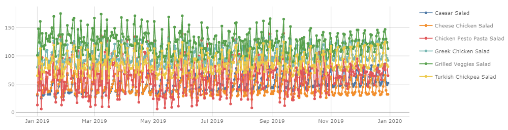
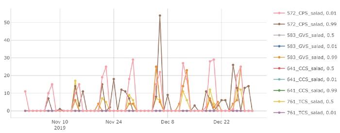
First, we merge the sales predictions to the existing sales store and plot the sales predictions for the 0.5 quantile for each salad against the timeline.
salad_cube.visualize("Sales for the whole year")
Now we assume that during our analysis we have an access to the storage capacity for the different products, we create a store from this newly available data and append it to the cube.
Let us use the information on the storage capacity and plot the storage capacity for each of the products based on the sales forecast of the 0.5 quantile.
Scenario creation
We create the scenarios for the sales prediction for the 0.99 and 0.01 quantiles. For the newly created scenarios, we calculate the available storage for three randomly chosen salad products.
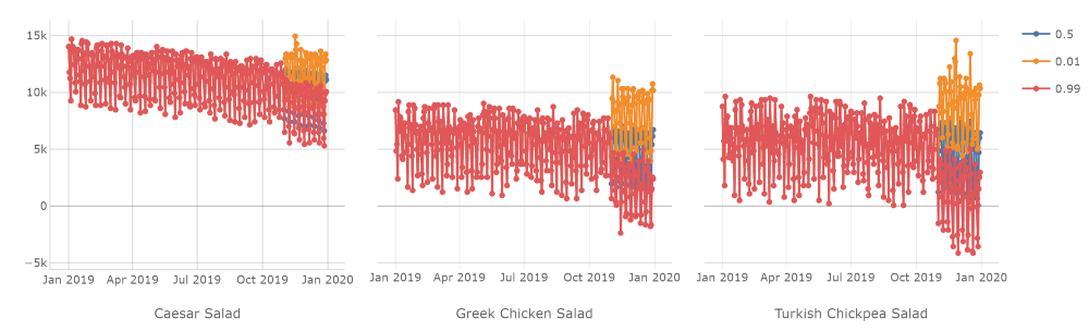
Observation: Here we can see that for many salads, we need additional storage (i.e. the available storage is negative) only in the case of 0.99 quantile of sales. For some products such as the Caesar salad, we do not need the additional space even for the 0.99 quantile of sale.
How to interpret these volumes?
There are two main ways to interpret these volumes:
- In terms of the number of excess products
- In terms of the number of refrigerators required
Let us discuss the above two methods in details:
- In terms of the number of excess products
m['excess_products'] = tt.agg.sum(tt.where(m['available_storage'] < 0,
tt.ceil(-m['available_storage']
/ m['product_volume']), 0),
scope=tt.scope.origin(lvl['prod_id']))
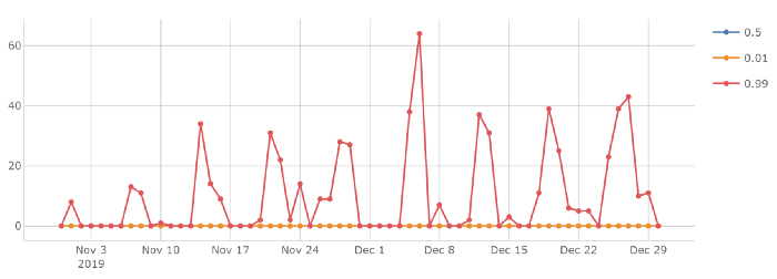
# visualizing the excess products
salad_cube.visualize("excess products for all quantiles")
Here we can see how many excess products we have given our current storage capacity against each of the quantile forecast scenarios of 0.99, 0.5, and 0.01 quantiles of sales. As expected the scenarios with 0.5 and 0.01 quantiles of sales have no additional products. Even in the scenario with 0.99 of sales, a few products like Caesar salad don’t need any additional storage space.
Insight — From the number of products to revenue:
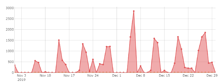
Now from each surplus product using the number of products and their respective sales price, we can calculate the total potential additional revenue.
The total potential additional revenue can be defined as the potential revenue we can generate if we can sell the products as per the 0.99 quantile of the sales prediction with no constraint on the additional storage available.
Thanks to Atoti, we can calculate and plot the total additional revenue by just a simple code
m['potential_additional_revenue'] = tt.agg.sum(m['excess_products']
        * m['selling_price.VALUE'], scope=tt.scope.origin(lvl['prod_id'
        ]))
2. In terms of the additional refrigerators
Since we already have the additional products and their corresponding volumes, we can calculate the total additional volume required. This can be simply converted into the number of refrigerators with an underlying assumption that the storage capacity of a refrigerator is 200 Litres.
Just one line of code and we can see the daily breakup of the additional number of refrigerators required.
From refrigerators to additional potential margin:
Although these refrigerators can bring in some potential revenues, they also have an operational cost. So with how many refrigerators is the net margin maximum? Is it even profitable to acquire some additional refrigerators? Thanks to Atoti, we can answer all these questions. Not only that, we can find the breakdown of the total costs and the total revenue for the scenarios with different numbers of refrigerators.
Here, we assume that the total daily operational cost of a refrigerator is 5 euros per day. And though there is no limit on the number of scenarios, for the sake of clarity we will compare the scenarios with 10, 15, 20, 25, and 40 refrigerators.
Q1 — How much of the total additional potential revenue can we actually realize in these scenarios.
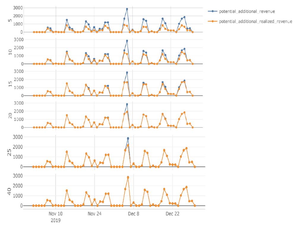
Here we can see, as we keep on increasing the number of refrigerators, there is an increase in the additional potential revenue which can be realized. With 40 refrigerators, we can realize almost the full potential revenue.
Q2 — But how much would it cost to the business?
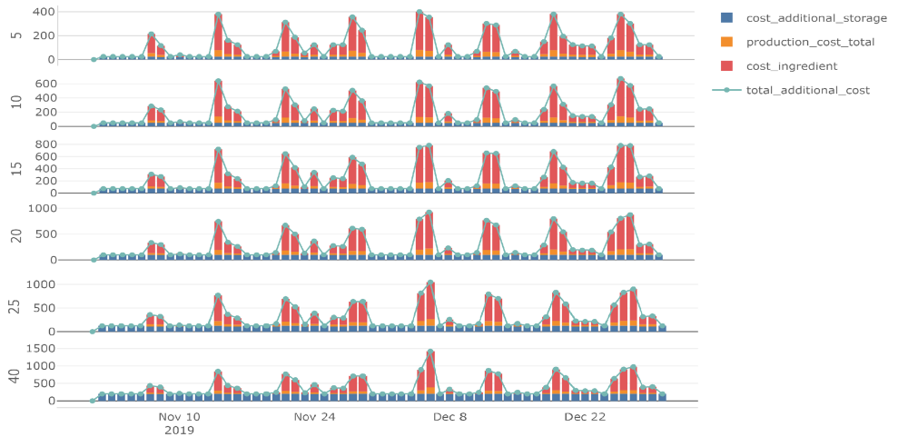
Intuitively, the total cost keeps on increasing as the number of refrigerators increases. The production and ingredients cost increase proportionally to the number of products being sold on that day while the additional storage cost being constant depending on the number of refrigerators.
Here is a comparison of the total revenue and the total cost for the cases with a varying number of refrigerators.
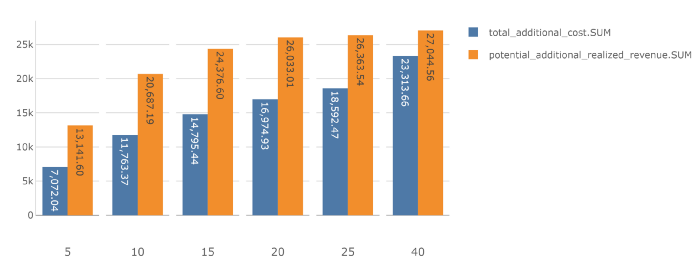
While having 40 additional refrigerators may materialize the full potential revenue, the return of investment ($3,730.90) is lesser than the rest of the scenarios. We can see that maximum revenue does not equate to the maximum margin in this case.
Q3 — So more potential revenue or less total cost, which scenario is the best?
We calculate the margin for the different scenarios and hence the one with the maximum positive margin will be our best scenarios.
Margin can be defined as the difference between the potential additional revenue realized and the total cost for that scenario.
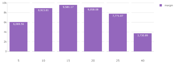
Hence, it can be concluded that in the scenario with 0.99 quantile of sales, we get an optimum additional margin by acquiring 15 additional refrigerators. So we should not be acquiring more than 15 refrigerators at the given daily operating price and the capacity of the refrigerators.
For the detailed source code and many other such interesting use cases, do check out the Atoti notebook gallery on GitHub.
Food for thought:
What would happen if the business could manage to acquire larger refrigerators at the same operating cost? And what if we could reduce the daily operational costs significantly?
Will it be still the same number of refrigerators for optimum margin?
Perform your own what-if analysis on the above use case and share it with us.