Translating ML output effectively to business terms for telecommunication

Attrition, also known as churn, is the loss of customers and it is a key metric for businesses that offer subscriptions and SaaS. These include financial services such as banks and insurance, telecommunication, internet service providers and pay-TV.

Impact of attrition

Churn tells us how departing customers affect the company’s monthly revenue and growth, which in turn impacts investors’ confidence in the company.

While it is important to acquire new customers in order to grow business, there are more perks that come with customer retention. Invesp has provided a good comparison between the two, showing that it can cost 5 times more to acquire new customers.

Understanding attrition in telecommunication

Advancement in technology and changes in users’ behaviour resulted in a high attrition rate for the telecommunication sector. Some contributing factors are:

• Mobile Number Portability (MNP), where customers can easily switch to another provider while preserving their number.
• Over-the-top (OTT) players such as Netflix, Amazon Prime Video, Disney+ which are bypassing the traditional operators’ network such as cable, broadcast and satellite television.
• OTT applications such as WhatsApp, Google Hangout, Skype which are cannibalizing the paid voice and messaging services.
• Frequent release of newer smartphones leading to less enticement to subscribe to mobile plans that last for a couple of years.
• No-contract plans that are data-heavy and price competitive by competitors, which attract high data usage consumers.

Predicting churn with machine learning

We can make use of predictive analytics to:

1. Determine the causal factors that may cause the customer to churn
2. Identify customers who have a higher probability of churning

By predicting the customers who are churning, businesses can come up with targeted retention strategies with the churn factors in consideration.

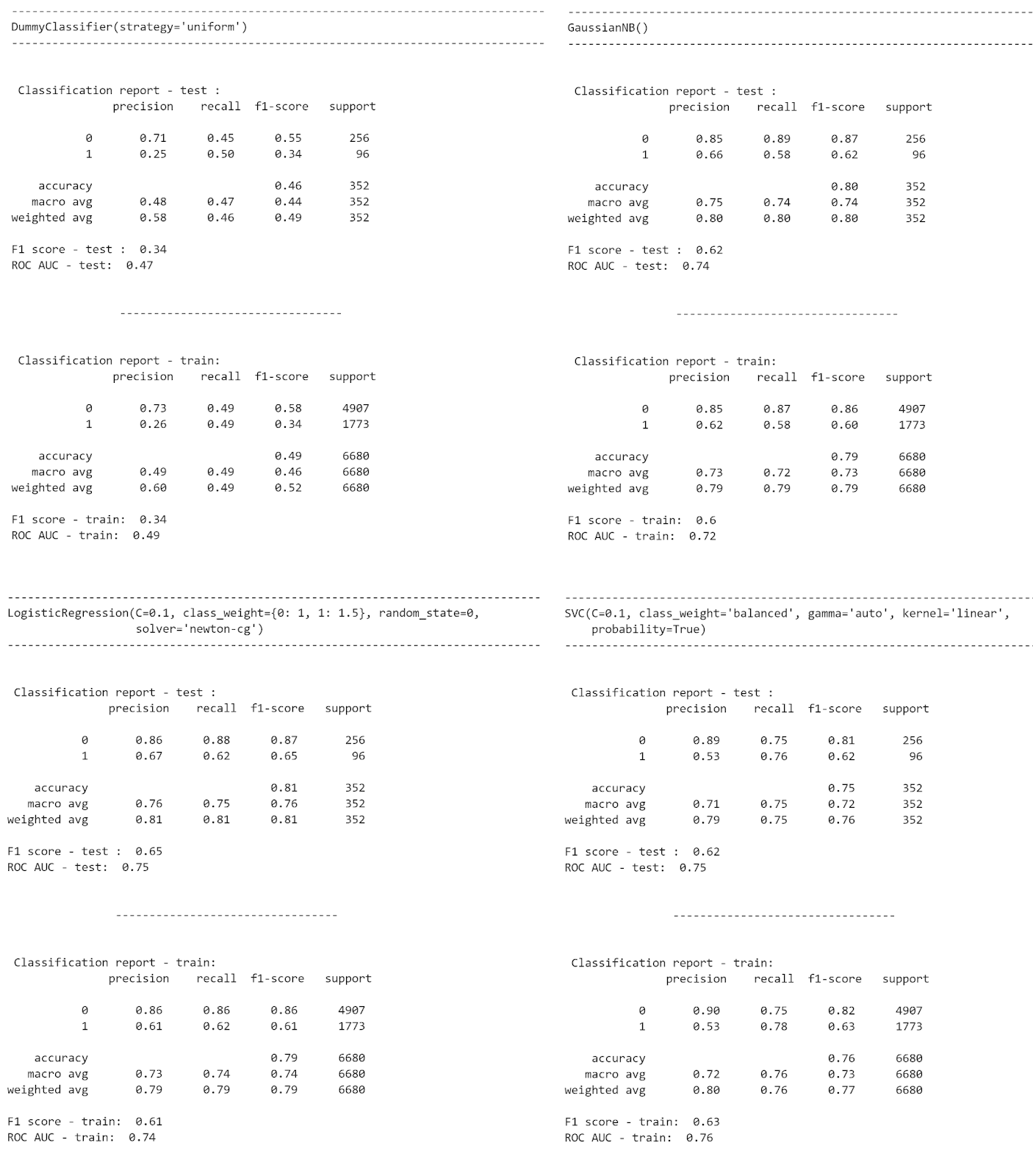
Instead of pondering over which model to use, we are going to explore and compare the churn predictions from four different models presented:

• Dummy Uniform Classifier
• Logistic Regression Classifier
• Naive Bayes Classifier
• SVM Classifier Linear Classifier

Translating churn prediction into business metrics

So what if we know who’s going to churn? We need to translate this prediction into useful metrics for business to draw insight from.

Research has shown that it can cost 5 times more to acquire new customers. Without considering expansion, how many customers should we attempt to retain?

1. All customers whether they will be churning
2. Either all or some of the customers who are predicted to churn
3. Randomly selected customers
4. None of the customers

The first option represents the ceiling of the retention budget by going all out while the second option largely depends on the accuracy of the churn model.

The third option is a game of luck without a strategy while the last option represents the ceiling of the acquisition budget by ignoring churn.

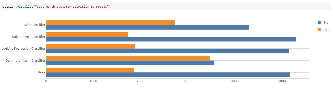
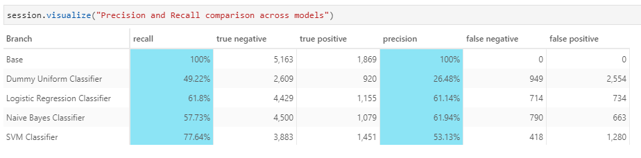
As we can see above, the number of churns predicted by different models varies greatly. This means that we could potentially be:

• Paying more than necessary to retain customers who are not churning
• Retaining far too few customers, consequently spending more money to acquire new customers

To draw the relevance to business, we will make use of the below business metrics in our analysis:

• Monthly Recurring Revenue (MRR) is the recurring revenue expected on monthly basis for the subscribed goods/services
• Net Revenue Retention (NRR) measures the change in the MRR over the period (includes benefits from expansion)

This article from HubSpot gives a good explanation of the above (termed slightly different).

Using NRR as a target metric, we will derive the following with the predictions from the four churn models:

1. The number of customers to retain
2. The customers whom the marketing team should try to retain
3. The retention and acquisition budget that business should allocate

The statistics above are computed based on a target NRR of 90% with a budget of $100 and $500 per customer for retention and acquisition respectively. What would also be interesting for business would be how the figures would change if:

• NRR target is adjusted
• Budget for retention and acquisition changes

We will be using the Telco Customer Churn data from Kaggle for machine learning and our analysis. You can access the source files below:

• Preparing data — transforming categorical variables into binary variables.
• Model creation — Training and saving different data models in pickle files.
• Data analytics — expense forecasting with machine learning predictions

Read on to find out how we can leverage Atoti’s multidimensional aggregation and simulation capability to derive useful business insights from the predictions of the churn models.

Step 1 — Load telco customer churn data into Atoti multidimensional data cube

After data preprocessing with Pandas, we can spin up a multidimensional data cube with Atoti as follows:

# a session has to be created for Atoti
session = tt.create_session()

customer_store = session.read_pandas(
    telcom, keys=["CustomerID"], store_name="customer_store", 
    types={"ChurnProbability": tt.type.FLOAT}
)

cube = session.create_cube(customer_store, "customer_cube")

We can start visualizing the data in the Jupyter notebook:

More than a quarter of the customers left the telco in the past month. The telco will lose all its customers in the coming months if this attrition rate keeps up.

Step 2 — Integrating machine predictions into the cube as a scenario

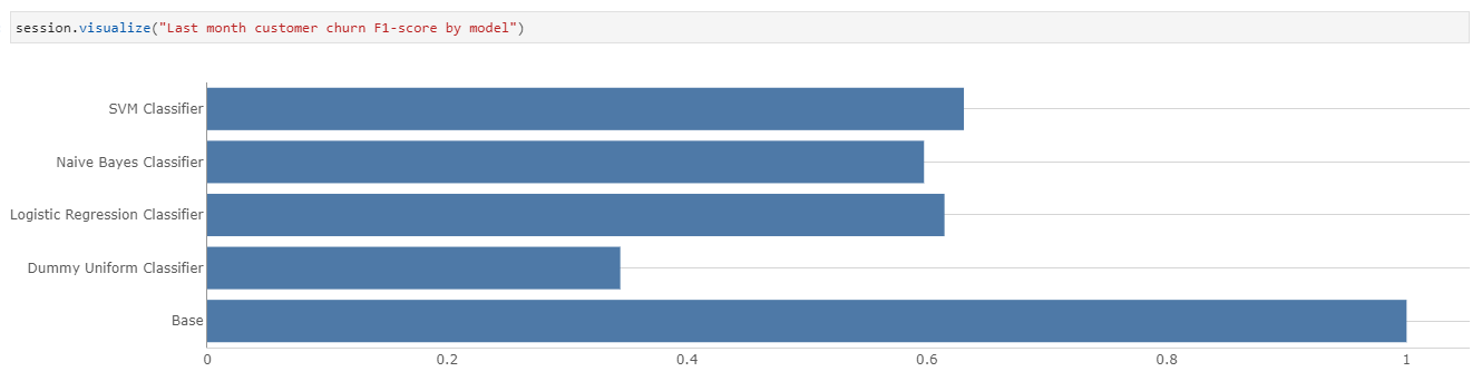
We see the below classification reports of the four models that we are going to compare in this article.

For each model, we get its corresponding prediction and probability on the test dataset using the predict and predict_proba function of the model:

gnb_prediction = gnb_clf.predict(test_X)
gnb_probability = gnb_clf.predict_proba(test_X)

We merge the predictions and probability of the test dataset back into the original dataset as follows:

• ChurnPredicted — Prediction output from the model
• ChurnProbability — Probability of churn happening (set the probability to zero if a customer is not predicted to churn)

def model_scenario(predictions, probabilities):

    churnProbability = np.amax(probabilities, axis=1)

    churn_forecast = telcom[telcom["Subset"] == "Test"].copy().reset_index(drop=True)
    churn_forecast = churn_forecast.drop(["ChurnPredicted", "ChurnProbability"], axis=1)

    churn_forecast = pd.concat(
        [
            churn_forecast,
            pd.DataFrame(
                {"ChurnPredicted": predictions, "ChurnProbability": churnProbability}
            ),
        ],
        axis=1,
    )

    # we are not interested in the probability if it is predicted that the client will not churn
    churn_forecast["ChurnProbability"] = np.where(
        churn_forecast["ChurnPredicted"] == 1, churn_forecast["ChurnProbability"], 0
    )

    churn_forecast["ChurnPredicted"] = np.where(
        churn_forecast["ChurnPredicted"] == 1, "Yes", "No"
    )

    return churn_forecast

We are now ready to load the model’s prediction back into the Atoti datacube!

Remember, we want to compare the performance of the models. To do so, we load the predictive output as a scenario in the datastore customer_store using Atoti’s source simulation.

customer_store.scenarios["Naive Bayes Classifier"].load_pandas(gnb_df)

With some simple measures creation, we can now compare the performance of the models in a pivot table:

Churn and MRR analysis

Let’s use a simple formula that uses the monthly recurring revenue (MRR) to compute the net revenue retention (NRR):

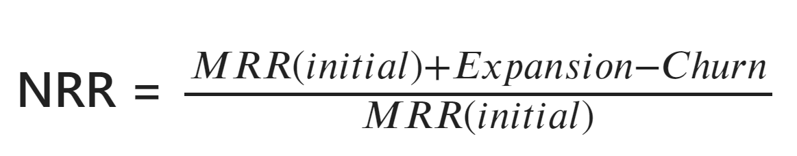
Churn is the revenue lost due to customers leaving. In this case, we do not consider the expansion of the business. See how we can create new measures for the MRR(Initial) and Churn to derive the NRR:

m["MRR Initial"] = tt.total(m["MonthlyCharges.SUM"], h["CustomerID"])

m["Actual RR Loss"] = tt.total(
    tt.filter(m["MonthlyCharges.SUM"], l["Churn"] == "Yes"), h["CustomerID"]
)

# we use ChurnPredicted here instead of churn because we want to see the difference between the prediction and the actual churn
# we know the exact amount of money (m["MonthlyCharges.SUM"]) lost if the customer churns
m["Predicted RR Loss"] = tt.agg.sum(
    tt.filter(m["MonthlyCharges.SUM"], l["ChurnPredicted"] == "Yes"),
    scope=tt.scope.origin(l["CustomerID"]),
)

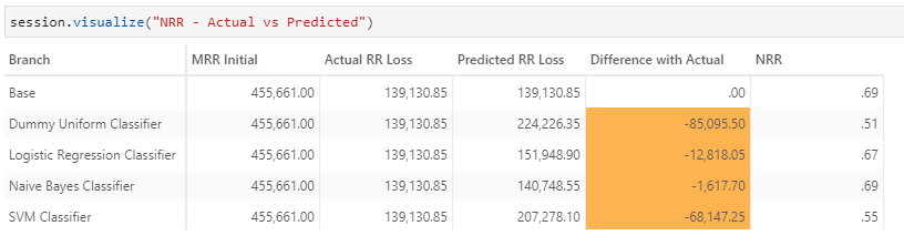
m["NRR"] = (m["MRR Initial"] - m["Predicted RR Loss"]) / m["MRR Initial"]

Note that the initial MRR should not be impacted by any filters, hence we use the `Atoti.total` function to get the total monthly charges across CustomerID. Also, pay attention to how we made use of filters on the levels `Churn` and `ChurnPredicted` to compute the actual and predicted loss.

We see in the below table that we could grossly overestimate or underestimate the loss if we are not careful with our projection, as in the case of SVM Classifier below.

Customer retention strategy

Let’s see some assumptions for our customer retention strategy:

1. We aim to achieve a target NRR of 90%
2. We compute the number of customers that we need to retain to achieve this target NRR
3. For each customer identified, we will set aside a budget of $100 for retention purpose
4. We do not know who has actually churned yet

Let’s start by creating a measure for the target NRR:

m["TargetNRR"] = 0.9

Computing the maximum possible loss in the revenue would allow us to achieve the target NRR:

m["Expected RR Loss"] = m["MRR Initial"] - (m["TargetNRR"] * m["MRR Initial"])

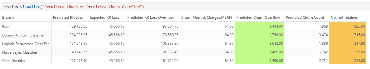
Predicted RR Loss Overflow is the amount of money between what we predicted we will be losing and the maximum loss we can have to achieve the target NRR.

The target revenue amount is the amount we need to obtain from the customers that are either to be retained or replaced.

m["Predicted RR Loss Overflow"] = tt.total(
    m["Predicted RR Loss"] - m["Expected RR Loss"], h["CustomerID"]
)

The average MonthlyCharges of those who are predicted to churn is used as the amount that each retained customer will give. By dividing the Predicted RR Loss Overflow by the average MonthlyCharges, we get the target number of customers to retain for each algorithm.

m["Churn MonthlyCharges.MEAN"] = tt.parent_value(
    m["MonthlyCharges.MEAN"],
    on=[h["CustomerID"], h["ChurnPredicted"]],
    total_value=m["MonthlyCharges.MEAN"],
    apply_filters=False,
)

m["Predicted Churn Overflow"] = tt.total(
    tt.math.ceil(m["Predicted RR Loss Overflow"] / m["Churn MonthlyCharges.MEAN"]),
    h["ChurnPredicted"],
)

The below measure Predicted Churn Count shows the number of customers is predicted to churn.

m["Predicted Churn Count"] = tt.agg.sum(
    tt.filter(m["contributors.COUNT"], l["ChurnPredicted"] == "Yes"),
    scope=tt.scope.origin(l["CustomerID"]),
)

Identifying customers to retain

Now that we have the retention size based on the average monthly churn charges, we need to identify who we want to retain. The easiest way is to retain those with the highest probability of leaving and have a monthly charge higher than or equal to the average.

Consider the scenario where we retained a customer whose monthly charge is $100: it would be equivalent to retaining 5 customers of $20 monthly charge.

Therefore, the strategy adopted is as follows:

1. We increase the churn probability for customers with a monthly charge greater than the average churn monthly charges
2. With Atoti.rank, we rank the customers who are churning based on the churn probability

# We only rank those customers who are churning. We give higher weightage to the customer with a higher charge so as to minimize loss
m["Churn Score"] = tt.where(
    (m["MonthlyCharges.MEAN"] >= m["Churn MonthlyCharges.MEAN"])
    & (m["ChurnProbability.MEAN"] > 0),
    m["ChurnProbability.MEAN"] + 1,
    m["ChurnProbability.MEAN"],
)

m["Churn Rank"] = tt.rank(
    m["Churn Score"], h["CustomerID"], ascending=False, apply_filters=True
)

Retention vs acquisition

Now that we have the ranking in preference for retention, we make further assumptions that for each customer retention, we will allocate a budget of $100. In the event we need to replace the customer, that would require a marketing budget of $500.

m["Retention budget"] = 100
m["New Customer budget"] = 500

So based on the ranking preference, we will do a forecast on the retention and marketing budget:

# we spent $100 on each of the customers identified and managed to retain all of them
m["Retention cost"] = tt.agg.sum(
    tt.where(
        (m["Churn Rank"] <= m["Predicted Churn Overflow"]) & (m["Churn Score"] > 0),
        m["Retention budget"],
        0,
    ),
    scope=tt.scope.origin(l["CustomerID"], l["ChurnPredicted"]),
)

# we retained none of the customers, hence spending $500 to recruit number of new customers equivalent to the Predicted Churn Overflow
m["New Customer cost"] = tt.agg.sum(
    tt.where(
        (m["Churn Rank"] <= m["Predicted Churn Overflow"]) & (m["Churn Score"] > 0),
        m["New Customer budget"],
        0,
    ),
    scope=tt.scope.origin(l["CustomerID"], l["ChurnPredicted"]),
)

Let’s see what kind of information these measures can give us.

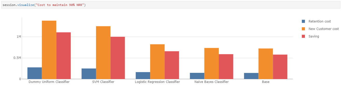
Assuming all the identified customers either get retained successfully or have to be replaced, we gather 2 information here:

• Naive Bayes Classifier costs the least to maintain 90% NRR, while the prediction based on SVM Classifier would be the most costly
• It would be a lot more cost-effective to retain customers than acquire new ones.

Reality check

We are ready to compare our forecast against the actual churn results!

We are going to assume that the retention budget offered is fully utilized, whether the customers had the intention to churn or not. This means that customers who had intended to churn got retained successfully.

# Churned customer targeted by the campaign
m["Successful Retention Cost"] = tt.agg.sum(
    tt.where(
        (m["Retention cost"] == 100) & (l["Churn"] == "Yes"), m["Retention cost"], 0
    ),
    scope=tt.scope.origin(l["CustomerID"]),
)

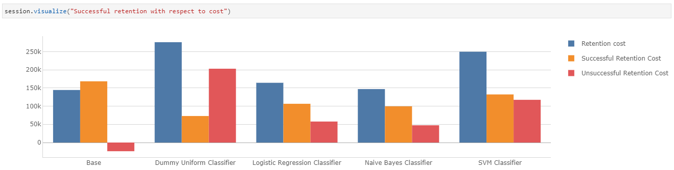
If we attempt to retain customers who have no intention of churning, the retention budget is wastefully utilized. Conversely, it is possible that some customers not targeted by our campaign actually churned and we probably would not achieve our target NRR.

# Churned customers that were not targeted by the campaign
# we know the actual amount that was lost through the lost of these customers
m["After Campaign RR Loss"] = tt.agg.sum(
    tt.where(
        m["Retention cost"] == 100,
        0,
        tt.where(l["Churn"] == "Yes", m["MonthlyCharges.SUM"], 0),
    ),
    scope=tt.scope.origin(l["CustomerID"]),
)

We have to spend more money to replace them, on top of the retention budget that we already spent.

Post retention NRR

On this basis, we compute the new NRR after the retention effort:

m["After Campaign NRR"] = (m["MRR Initial"] - m["After Campaign RR Loss"]) / m[
    "MRR Initial"
]

There we have it!

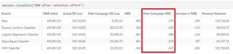
After the retention campaign, NRR for all models reached above the target of 90%. The revenue retained with SVM Classifier is the highest! This is natural, considering the model has a larger target base of 2,496 customers compared to the rest. This translates to higher unsuccessful retention and expenses.

Customer acquisition to reach target NRR

So after a round of retention effort, we need to acquire new customers if we haven’t reached our NRR target.

Let’s compute the gap in NRR and the number of customers we estimate to acquire.

gap_to_target_nrr = m["TargetNRR"] - m["After Campaign NRR"]

m["Gap in revenue loss"] = m["After Campaign RR Loss"] - m["Expected RR Loss"]

m["Clients to replace"] = tt.total(
    tt.where(
        m["Gap in revenue loss"] > 0,
        tt.math.ceil(m["Gap in revenue loss"] / m["Churn MonthlyCharges.MEAN"]),
        0,
    ),
    h["ChurnPredicted"],
)

We can compute the marketing budget required for the acquisition of the new customers:

m["Actual New Customer budget"] = m["Clients to replace"] * m["New Customer budget"]

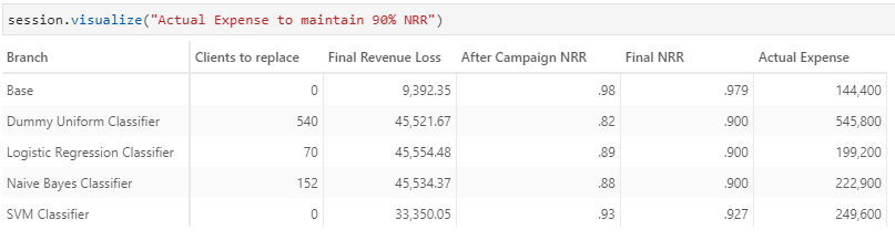
Since the retention budget is already spent, we have to add it to the marketing budget to compute the actual expense for us to reach the target NRR.

m["Actual Expense"] = m["Retention cost"] + m["Actual New Customer budget"]

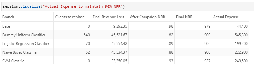
The figures showed that the Logistic Regression Classifier would be the most cost-effective model to achieve the target NRR of 90%!

Alternative situations

What if we want 95% NRR?

Curious to know how the figures would change if the target NRR is changed? With Atoti’s what-if feature, we can do so simply by creating a measure simulation that allows us to replace the TargetNRR value:

NRR_simulation = cube.setup_simulation(
    "NRR Simulation",
    base_scenario="90% NRR",
    replace=[m["TargetNRR"]],
).scenarios

In this case, we replace the NRR from 0.9 to 0.95.

NRR_simulation["95% NRR"] = 0.95

Without further processing, we can compare the difference between 90% and 95% target NRR through Atoti visualization:

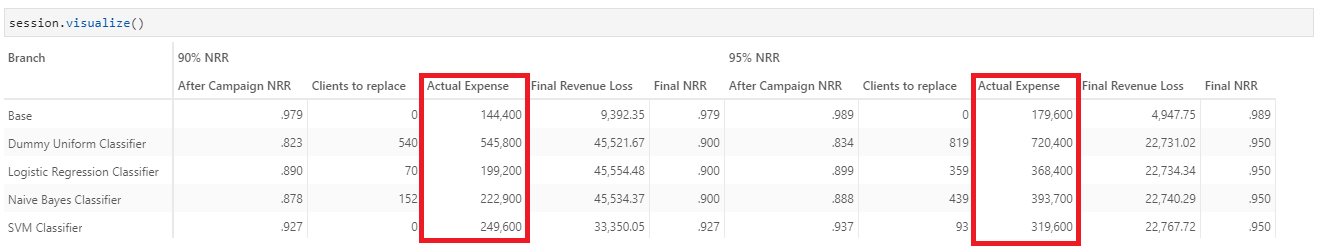
Logistic Regression Classifier is still the most cost-efficient algorithm.

What if the marketing budget is twice the expected

Instead of replacing the value of measures in the simulation, let’s create a simulation that scales a measure instead:

marketing_budget_simulation = cube.setup_simulation(
    "New Customer budget Simulation",
    base_scenario="5 x Retention",
    multiply=[m["New Customer budget"]],
).scenarios

We will multiply the Marketing budget by 2 to see how the total expenses will be impacted:

marketing_budget_simulation["10 x Retention"] = 2

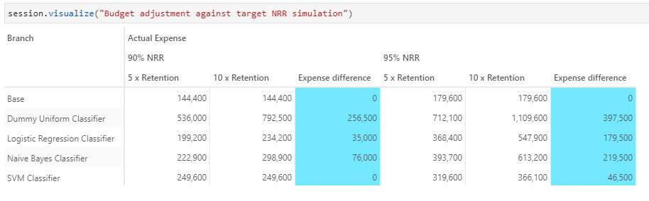
We see SVM Classifier is unaffected by the increase in marketing budget, as the retention effort is sufficient to maintain the 90% NRR. However, the expenses for target 95% NRR more than doubles that of 90% NRR.

What’s next?

We saw how Atoti can help in business decision making, as well as analyse the accuracy of machine learning models. With longer periods of data, we could imagine having better model training and improvement on the accuracy of the prediction.

Also, we have not considered the features’ importance in this article, and have only taken into account the monthly charge. We can imagine identifying customers for retention based on the services or demographic and applying different retention budgets accordingly.

We welcome you to share with us how you would implement your customer retention strategy!