I am a quantitative analyst for ActiveViam. In this blog, I will provide an example of how to use Python to launch an in-memory analytics app to compute the cumulative rate of return interactively. You can download this example and play with it locally. It should be quite easy to modify it to fit your input data and the formula.

Introduction

In recent years, the application of advanced analytics for asset management has started demonstrating its value. Having the ability to dynamically compute performance analytics is one example. (As McKinsey & Company writes in this paper:  “Advanced analytics in asset management: Beyond the buzz”). 

Long gone are the days when it was easy to compute portfolio performance metrics.  Different kinds of asset types have sprung up in multiples and the portfolio construction process has become more complicated. Today, portfolio managers might want to understand what is driving the portfolio’s return and carve out strategies or groups of securities through specific time periods to answer client inquiries or run back-tests.  

The problem of performance calculation becomes harder when the methodology is non-linear. This means that it is not possible to precompute components of the formula to speed up the calculation. Instead, you have to compute the measure from the granular inputs to achieve a precise result.

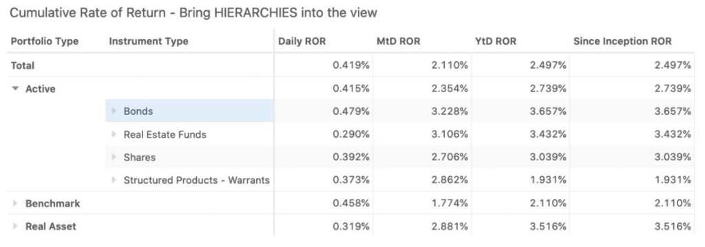
In this recording, the cumulative profit and loss (PL) metrics are recomputed interactively as I change the scope of data in the view – filtering based on date selection, and data expansion by Instrument Types, Portfolio Types and Countries.

You could sacrifice flexibility and adopt a simpler formula or accept the fact that performance is pre-calculated based on certain predefined strategies or portions of a portfolio.

For portfolio analysts who are dissatisfied with these compromises, this blog offers a  different approach that enables users to interactively recompute performance measures from the granular data using an in-memory technology. With this approach, you can perform quick calculations on a big data set and analyze performance metrics with any combination of attributes to achieve a more in-depth view of investment performance.

The recipe

I invite you to review this Python notebook, it allows you to launch a BI app powered by in-memory technology that will illustrate how cumulative performance metrics can be computed interactively.

The sample data included in this example contains 2 years of observations of daily PnL and investments for a few portfolios at instrument level. This is a small dataset I generated to support the example. Please refer to the blog by Alexis Blervaque where we applied the same technology on a bigger dataset: “Case study: How we implemented interactive portfolio return analytics on 60 bln data points“.

As an example of a cumulative performance metric I’ll use the following expression:

In this formula there’s a product over date of the rate of return (RoR) plus 1. You can use the product with summation, and the rate of return with other types of profit-and-loss metrics.

As illustrated in the GIF above, when users drill in and drill up, the system will recompute cumulative RoC. For each cell in the view, the calculation starts by summing up profit and losses  and total investment for the cell, then the return is calculated, and finally, cumulation over dates.

It would not be possible to roll-up the Cumulative PnL in any other way due to the nature of the formula, as the RoR is not additive:

Start by loading the data into Atoti, a Python library which I used to create a BI analytics platform. The components of the above formulae are easily defined via the python API. See, for instance, how the RoR metric is defined:

m["Daily ROR"] = m["Profit and Loss.SUM"] / m["Investment.SUM"]

The expression for the cumulative RoR calculation uses “scope” type “cumulative” as a parameter:

m["Cumulative ROR"] = (
    tt.agg.prod(
        m["Daily ROR"] + 1,
        scope=tt.scope.cumulative(l["Day"]),
    )
    - 1
)

Now when the formulae are defined, they are abstracted from the attributes, meaning, you can combine these measures with any dimensions that exist in your data and the formula will be recalculated.

In the notebook referred to in this blog, you will find the syntax for the MtD, YtD PnL cumulations, and a way to allow users to select arbitrary date periods.

Conclusion

The performance analytics in this blog is an example of a non-linear calculation, a problem that we deal with everyday – check my other blog posts on Value-at-Risk and other calculations.

If it is not possible to pre-compute the metric for any possible slice of data, give Atoti a try, as it enables quick recalculation of complex measures based on user query.