Counterparty credit risk analytics and what-if

In this post, I will show how you can implement an interactive analytical app for SA-CCR analytics in python using Jupyter Notebook and Atoti. You can take this example as a starter, and adapt it to your data model or adjust the calculation logic, for instance, to enable sensitivity-based AddOns.

As a quick reminder, the SA-CCR is a regulatory methodology for computing EAD (Exposure At Default) which is part of the consolidated Basel framework. It is already implemented for financial institutions in Europe by the Regulation (EU) 2019/876 (CRR II) and will be applicable from June 2021 and January 2022 in the US. In this post, I will walk you through the calculations as defined in the BCBS 279 document.

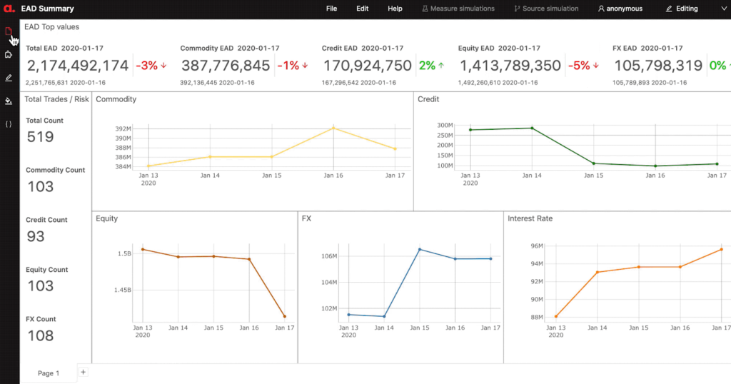
Here is an example showing a dashboard built in Atoti for SA-CCR. Continue reading to learn how to implement on-the-fly EAD calculations and What-If simulations.

Why Atoti

Atoti is an excellent tool for subject matter experts who wish to create analytical applications from a python notebook. It will automatically launch a web-based user interface to visualize the results. The dashboards can be shared with other teams, at any stage of the model development. The new calculations can even be accessed directly from Excel. An application implemented in python can be put in production.

You will see later in this post, how we can define complex aggregation functions in python — such as option’s delta adjustment as an example — and the calculations will be applied to the input data on-the-fly, so we can explore, interactively recompute and slice-and-dice the metrics in Atoti app.

The example dataset used has only a handful of positions, but the backend can scale linearly to handle terabytes of data. This is particularly useful, as in order to validate the calculations I may need to inject the entire derivatives book and view the numbers on the different levels — from netting set to counterparty or to a legal entity or to the global portfolio. Even with terabytes of data and having appropriate hardware, I can navigate through the portfolio and visualize the risk numbers at a sub-second query response time. You can read more about the technology behind Atoti in this white paper.

Finally, Atoti encourages experimentation and what-if analysis, as it provides a powerful simulations framework that can be used to test interactively the impact of a new trades in the capital requirement or estimate the impact of trading a new derivative on a list of counterparty so immediately we would know which counterparty will be the “cheapest to deal with”. Another example is a simulation of a change of regulatory input parameter. Could be useful in this time when local regulators could eventually change the supervisory parameters.

Getting started

To get started, please review this article as it explains how to download and install the Atoti python module.

Even if you are new to python, I encourage you to review the code and I’ll do my best to explain the process so that you are well-equipped to implement the calculation locally, customize it and extend.

Downloading the notebook example

You can download and run the example notebook discussed in this post from our gallery: SA-CCR notebook.

What to expect?

In the notebook you can find code snippets implementing the following calculation steps from the CRE52:

• Supervisory duration — [52.34]
• Trade-level adjusted notional (for trade i): di — [52.34]
• Maturity factors — [52.48] — [52.53]
• Supervisory delta adjustments — [52.38] — [52.41]
• Trade Effective Notional — [52.30]
• Asset class level add-ons — [52.55]
• Aggregate add-on — [52.24]
• Multiplier — [52.23]
• PFE add-on for each netting set — [52.20]
• Replacement cost — [52.10]
• EAD — [52.1]

Later In this post, we’ll discuss an example of the Delta Adjustment and you can find all other measures in the notebook.

We’ll also discuss contributory measures — using an example of “Pro-rata” allocation. And then we’ll look at how to configure simulations — on Supervisory Parameters What-If and CSA changes.

How to build an SA-CCR app?

Every analytical app in Atoti can be built in three steps:

• Launch Atoti
• Inject and link together the data
• Define measures

Having completed the above steps, you can start analysing your portfolio and perform simulations. Let me walk you through an example.

Launching Atoti

The first thing we need to do is to import Atoti and launch the app, we can do so using the following code cell:

import Atoti as tt
session = tt.create_session(name = "main session", config='./configuration.yaml')
session.url

At this stage, the web application is already running and Atoti is ready to consume data and aggregation logic.

Input data

In our example, the following data stores will be used as inputs to the calculation and we’re sourcing csv files saved on s3 to populate the stores:

• trades_store with information on the trades, their notionals, market values and time period parameter dates — Mi, Ei, Si and Ti [52.31]
• nettingSets_store — providing netting set attributes, such as MPOR and collateral, isMargined attribute and others
• supervisoryParameters_store — values set in section [52.72] “Supervisory specified parameters”.

The following code snippet is an example creating the trades store — we’re specifying the key fields and the data types:

trades_store = session.read_csv(
    "s3://data.Atoti.io/notebooks/sa-ccr/inverted/trades_preprocessed/trades_preprocessed_2020-01-13.csv",
    keys=["AsOfDate", "TradeId"],
    types={
        "Notional": tt.types.DOUBLE,
        "MarketValue": tt.types.DOUBLE,
        "AsOfDate": tt.types.LOCAL_DATE,
        "Mi": tt.types.LOCAL_DATE,
        "Si": tt.types.LOCAL_DATE,
        "Ti": tt.types.LOCAL_DATE,
        "Ei": tt.types.LOCAL_DATE,
    },
)

The read_csv is just one way of uploading the data, please refer to the doc to learn more about input data sources.

Linking the data — snowflake

Having loaded the csv files into datastores as described above, I am linking them to create a “snowflake” data model, where every other store is enriching the main — trades_store:

trades_store.join(
    nettingSets_store, mapping={"NettingSetId": "NettingSetId", "AsOfDate": "AsOfDate"}
)
trades_store.join(
    supervisoryParameters_store,
    mapping={"AssetClass": "AssetClass", "SubClass": "SubClass"},
)

As a next step, we’re creating the cube. Usually Atoti’s create_cube command creates .SUM and .MEAN measures automatically from numerical data inputs, to prevent that we’re running the command will the mode = no_measures.

cube = session.create_cube(trades_store, "SA-CCR", mode="no_measures")

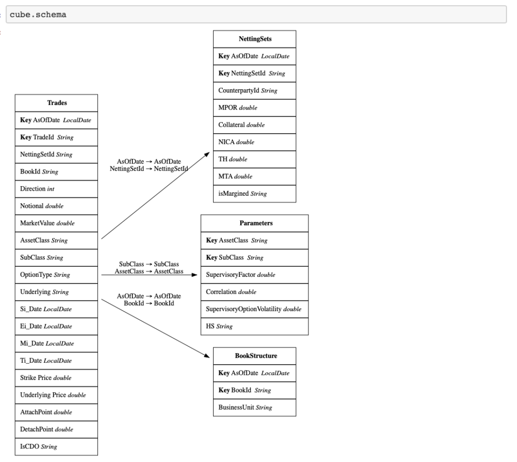
The cube.schema will display the current state of the data mode inside the notebook.

Defining the SA-CCR measures

Having defined the data model, we can start creating the measures to compute SA-CCR measures on-the-fly from the input data.

To summarize the calculations, I made this flowchart: the white circles represent input data, the red ones — represent Atoti on-the-fly calculations:

As you can see from the diagram, the EAD measure is implemented with a chain of interim measures — taking into account the effects of duration, maturity, delta adjustments, correlations between risk factors for the individual asset classes, effects of collateral — which are calculated every time a user visualizes the portfolio.

Please refer to the notebook to find code snippets for each of the “bubbles”. Here let me give you an example for the “Delta Adjustment”.

Depending on a trade, the “Delta Adjustment” will use a different formula:

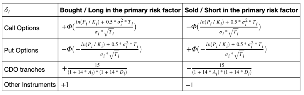
We will compute the “Delta Adjustment” measure as a product of the following multipliers, each computed per the above formulae for the relevant trade or takes the value of 1 otherwise:

m["Delta_Adjustment"] = (
    m["Direction"] * call_multiplier * put_multiplier * cdo_multiplier
)

In this formula, the measure m[‘Direction’] takes the values of 1/-1 for long/short positions, and multipliers are computed using Atoti’s “where” expression:

call_multiplier = tt.where(lvl["OptionType"] == "C", CDF(m["d"]), 1.0)
put_multiplier = tt.where(lvl["OptionType"] == "P", -CDF(-m["d"]), 1.0)
cdo_multiplier = tt.where(
    lvl["IsCDO"] == "Y",
    15.0 / ((1.0 + 14.0 * m["AttachPoint"]) * (1.0 + 14.0 * m["DetachPoint"])),
    1.0,
)

The CDF in the options adjustment formula is defined using Atoti math’s error function:

def CDF(x):
    return (1.0 + tt.math.erf(x / tt.sqrt(2))) / 2.0

I wrapped the argument of the CDF function into the following Atoti measure:

m["d"] = (
    tt.log(m["Underlying Price"] / m["Strike Price"])
    + 0.5 * (m["Supervisory_Option_Volatility"] ** 2) * m["Ti"]
) / (m["Supervisory_Option_Volatility"] * tt.sqrt(m["Ti"]))

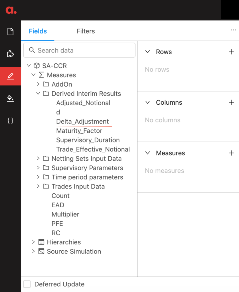
Once we defined the “Delta Adjustment” measure in Atoti, users can select it from the cube explorer and visualize in a dashboard:

If you want to look at AddOns, PFE, RC and other calculations feel free to download the SA-CCR notebook in Atoti gallery.

What-If on supervisory parameters

So far we’ve discussed how to create an app for the SA-CCR calculations and visualization. Such an application allows to slice-and-dice EAD and interim measures, and visualize them in a view.

To make the tool more powerful for users, you can set up “simulations” — to allow users to experiment with calculation parameters or upload alternative data sets — and evaluate the impact instantaneously side-by-side with the original version.

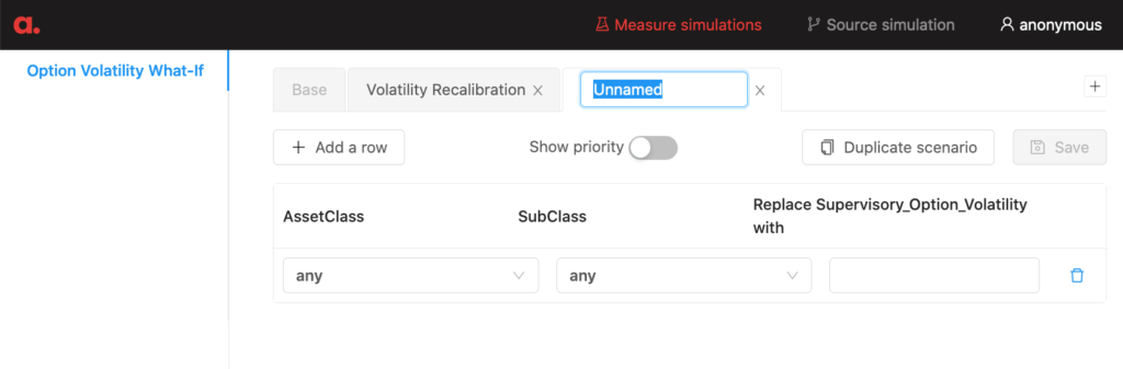
For example, “Measure simulations” feature in Atoti allow to configure “replace”, “multiply” and “add” actions on measures. In our case, let’s create a simulation to replace volatility values for different AssetClasses as follows:

param_what_if = cube.setup_simulation(
    "Option Volatility What-If",
    replace=[m["Supervisory_Option_Volatility"]],
    levels=[lvl["AssetClass"], lvl["SubClass"]],
)

Having setup the simulation, we apply the changes we want in our experiment.

recalibration = param_what_if.scenarios["Volatility Recalibration"]
recalibration += ("IR", "No SubClass", 0.1)

The end-users can add “what-if” scenarios through the UI:

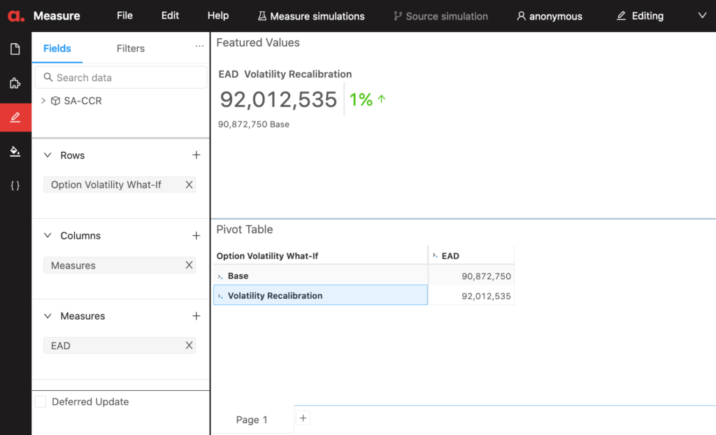
To evaluate the impact of changes on the EAD, it can be broken by the scenario in a view:

In addition to the “Measure simulations” — you can also apply “Source simulations” — which allow uploading alternative data sets. In my notebook, you can find an example of updating CSA attributes.

Conclusion

In this post, we discussed how to create an SA-CCR app in Atoti. This example can be adjusted for your data and the methodology, for instance, the delta calculation in the EBA approach has to take into account the sensitivities.

In my future posts, I want to discuss another aspect of the SA-CCR — non-linearity and allocation metrics — stay tuned!