IFRS 9 portfolio analytics with Atoti

This blog provides a guide on how to address daily credit portfolio monitoring needs, in particular to track and explain expected credit losses for IFRS 9, perform vintage analysis, drill-down to loan-level data, analyze changes between periods and determine the main drivers behind the portfolio risks. 

I will furnish you with a step-by-step outline on how to build an IFRS 9 analytical app in Python using a Jupyter Notebook and Atoti. 

By way of regulatory background, as a result of the 2007-2008 global financial crisis, accounting standards were redesigned and the International Financial Reporting Standard number 9 (IFRS 9) and Current Expected Credit Loss (CECL) were introduced. A key tenet of the regulation is  the requirement to recognize in financial statements not only the incurred losses for a credit portfolio, but compute a forward-looking measure – expected credit losses (ECL) for a portfolio. The ECL computation relies on the three metrics: probability of default (PD), loss given default (LGD), and exposure at default (EAD).

Python implementation

You may download the Jupyter Notebook that implements the IFRS 9 app in Python (the link is below). I’m using the Atoti Python module to launch an in-memory aggregation engine and a reactive UI for end-users to visualize and understand credit portfolio risk metrics. It comes with a free limited license so you can run it on your own. 

I’ve created a sample data set based on the Lending Club dataset available on Kaggle and mocked-up the risk engine outputs – PDs, LGDs, EADs, Stage classification – to illustrate how the IFRS 9 metrics can be computed and explored in an analytical app.

Here’s the link to the example Jupyter Notebook on GitHub:  IFRS 9 analytics with Python and Atoti, you can simply run all cells to launch the BI app with our reference data on your laptop. 

You can take the example referred below as a starter, and adapt it to your data model or adjust the calculation logic. Let me explain the main implementation steps.

Step 1 Installation

To run the notebook, you will need to install Atoti Python module. See the installation instructions here. Atoti comes with a free community edition limited license.

Step 2 Creating a session

As illustrated in the notebook, after importing the Atoti module you need to create a session. At this stage an in-memory cube is started and the user interface is running. You can access the user interface by running session.url – the app is already running, but there’s no data:

The notebook can be deployed on a server, then your colleagues can access the application via a URL, explore the portfolio and build dashboards. Please refer to the “IFRS 9 Data Viz” section of this series for examples of dashboards and data visualizations.

Step 3 Loading Loan-level data

Once the session has been created, the app is already running, but there’s no data. Let’s inject the contracts’ information and risk metrics.

We want to allow our users to explore IFRS 9 portfolio metrics interactively and slice-and-dice them by various attributes. The data inputs in our example include:

1. risk_engine_data keeps information on the individual loans, their explosures, stages, credit risk parameters for ECL calculation and other attributes by date,
2. lending_club_data keeps additional data – client attributes, such as grade (rating) and loan purpose, as well as most recent loan status,
3. loans_at_inception is storing loan opening information, such as opening date and opening risk characteristics. 

Each of the data stores in the reference example is loaded from a csv file, for instance the contract-level details are loaded using Atoti “read_csv” function:

risk_engine_data = session.read_csv(
    "lending-club-data/risk-engine/",
    keys=["Reporting Date", "id"],
    store_name="Credit Risk"
)

The columns of the newly created datastore are inferred from the input data, and we specify the key columns, store name and other parameters. You can read more about data loading and other data formats available in the Atoti documentation.

Having loaded all the necessary data inputs, we link them together using the “join” command:

risk_engine_data.join(lending_club_data)
risk_engine_data.join(loans_at_inception)

Finally, let’s run the “create_cube” command to get the dimensions populated in the UI:

cube = session.create_cube(contracts_store, 'IFRS9’)

This way we have just defined a snowflake type of data model. The data will be joined “on-the-fly” every time a user displays a measure and breaks it down by a column available in the “leaf-stores”.

Having run the “create_cube” column, we can start visualizing the data by selecting fields in the user interface:

You can inject more data into the existing datastores or add additional ones at any point later. Now let’s define the ways to aggregate portfolio data.

Step 4 On-the-fly portfolio calculations

In the previous step we have loaded contract-level risk inputs. Now let’s define metrics for portfolio analytics. 

You can find code snippets for various IFRS 9 portfolio measures in the Notebook referred above, including:

– the Stage and the Previous Stage, Stage Variation Indicator

– Previous EAD and Changes

– PD, Previous PD, Opening PD, PD Variation

– ECL

We use the Atoti Python interface to define the aggregation formulas, and the Python code gets translated into a Java post-processor that will compute the required expression from the granular contracts data – every time the user displays a metric in a dashboard. We can filter/slice-and-dice the metric in the user interface – in other words change the scope of data as we want – and the aggregation engine will recompute the expression interactively.

Now I’d like to discuss  the implementation of a particular IFRS 9 measure – the Expected Credit Loss –  and its Explainers. We will implement the ECL from loan-level LGD, EAD and PD, so that we can manipulate the inputs and easily decompose the portfolio ECL variation into the main drivers. 

Portfolio Expected Credit Loss

In the reference example, we compute the Expected Credit Loss (ECL) from pre-classified loan-level LGD, EAD and PDs. The Expected Credit Losses are recognized according to the stages per following formulas:

IFRS Stage 1: ECL=EAD*PD 12M*LGD

IFRS Stage 2: ECL=EAD*PD LT*LGD

IFRS Stage 3: ECL=EAD*LGD

To implement the above calculations, we use Atoti “sum_product” aggregation function. Firstly, three ECL formulas are configured depending on the stage:

ecl_stage_1 = tt.agg.sum_product(
    risk_engine_data["LGD"], risk_engine_data["EAD"], risk_engine_data["PD12"]
)
ecl_stage_2 = tt.agg.sum_product(
    risk_engine_data["LGD"], risk_engine_data["EAD"], risk_engine_data["PDLT"]
)
ecl_stage_3 = tt.agg.sum_product(risk_engine_data["LGD"], risk_engine_data["EAD"])

The Atoti “sum_product” aggregation function will multiply the EAD, PD and LGD (if applicable) for each individual contract, and sum up across contracts. Having defined the formula for each stage, it’s applied to contracts depending on which stage they belong to:

m['ECL']  = tt.filter(ecl_stage_1, l['Stage'] == 1) + tt.filter(ecl_stage_2, l['Stage'] == 2) + tt.filter(ecl_stage_3, l['Stage'] == 3)

We have just created a measure to compute Expected Credit Loss from PD, LGD and EAD.

Day-to-day variations

Let’s create measures displaying the previous ECL and daily changes. Using the “shift” function, we can display ECL for the previous day:

m['Previous ECL'] = tt.shift(m['ECL'], on=l['Reporting Date'], offset=1)

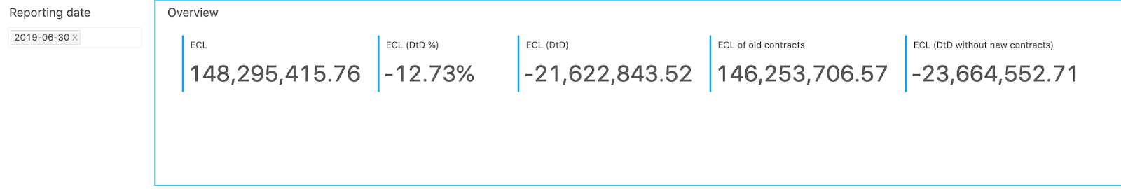
Having created the measure for the previous day ECL, let’s configure the DtD calculation, we just need to check that the previous value is valid for the calculation:

m['ECL (DtD)'] = tt.where(m['Previous ECL'] != None, m['ECL'] - m['Previous ECL'])
m['ECL (DtD %)'] = tt.where(m['Previous ECL'] != 0, m['ECL (DtD)'] / m['Previous ECL'])

For convenience, we can compute the DtD change for a portfolio as if there were no new contracts. Let’s filter out new contracts using Atoti “filter” function:

m["ECL of old contracts"] = tt.filter(m["ECL"], l["Reporting Date"] != l["issue_date"])

Having defined the “old contracts” this way, we can compute the DtD change excluding the impact of new contracts:

m['ECL (DtD without new contracts)'] = tt.where(m['Previous ECL'] != None, m['ECL of old contracts'] - m['Previous ECL'])

ECL Explainers

As discussed earlier, we have chosen to aggregate the ECL from the loan-level LGD, PD and EAD. This way, we can compute the variations due to these factors by comparing the loss calculation with calculation as if PD, LGD or EAD were the same as yesterday. 

Here’s an example for the ECL variation due to PD changes, and you can find the code snippets for the other two factors – LGD and EAD – in the notebook referred above.

The first thing, we need to calculate ECL using the PDs from the previous day as follows:

ecl_pd_explain_stage_1 = tt.agg.sum_product(contracts_store['LGD'], contracts_store['EAD'], previous_contracts_store['Previous PD12'])
ecl_pd_explain_stage_2 = tt.agg.sum_product(contracts_store['LGD'], contracts_store['EAD'], previous_contracts_store['Previous PDLT'])

ecl_with_previous_pd = tt.filter(ecl_pd_explain_stage_1, l['Stage'] == 1) + tt.filter(ecl_pd_explain_stage_2, l['Stage'] == 2) + tt.filter(ecl_stage_3, l['Stage'] == 3)

Then the variation attributed to the change in PD is simply a difference between the actual ECL and the ECL computed using the previous day’s PDs:

m['ECL variation due to PD changes'] = m['ECL'] - ecl_with_previous_pd

The percent of DtD change explained by PD can be configured as follows:

m['ECL variation due to PD changes (%)'] = m['ECL variation due to PD changes'] / m['ECL (DtD)']

This was just a few examples of the analytical measures that you can create. Check more examples in the Notebook.

Conclusion

What is novel about Atoti is that it’s fairly easy to get started and quickly create a BI app powered by an in-memory aggregation engine with a reactive UI from a Jupyter Notebook. The Python interface of Atoti empowers subject matter experts to implement the analytics as they want. At the same time, the application built through the Atoti Python interface is a Java application. Once you are happy with it, integrating the model into a scalable production environment and plugging in target data sources including real-time messaging systems is easy. For enterprise deployments with additional features such as role management and dedicated support, you may want to look up the commercial version of Atoti, Atoti+.

In the next blog post – “IFRS 9 Data Viz: ECL, PD Analytics and the Vintage Matrix” – we will build dynamic pivot tables, dashboards, and perform vintage analysis. Stay tuned!