Given a portfolio and an optimizer, can we find a ‘better’ portfolio using Atoti?

It’s a classic situation: you versus a benchmark portfolio. Maybe you’ve built your own portfolio optimizer or maybe you found an optimizer online. Either way, once you have your optimized portfolio output (or outputs!), you still need to compare it against the benchmark. But how?

In this article (part one of a three part series about Portfolio Optimization), we demonstrate how to integrate an external portfolio optimizer with Atoti to perform a benchmarking comparison on our equities portfolio. 

Read on to learn how we can build an initial solution. Check back in a few weeks for the rest of the series, and learn how to construct portfolios subject to various constraints that minimize CVaR, and explore how to perform portfolio rebalancing.

Let’s go!

Background

Let’s assume we have a portfolio with a set of initial weights for each instrument. Here, we are working exclusively with stocks (but you can choose your asset class). 

For each instrument, we’ve downloaded 3 years worth of data from Yahoo Finance using the yfinance library.

We use iPyWidget to enable an interactive selection of the portfolio we want to optimize, simplifying the experience to upload an initial portfolio. This initial portfolio is loaded into an optimizer which will return updated weights for the existing instrument in the portfolio based on several optimization options. The weights are then loaded back to Atoti to create a distinct portfolio option. In this example, we use the Python API PyPortfolioOpt to perform the optimization. This library provides five options for portfolio optimization:

• Based on maximal Sharpe Ratio (max_sharpe)
• Based on Custom nonconvex objectives (nonconvex)
• Based on Hierarchical risk parity (HRPOpt)
• Based on Critical Line Algorithm (CLA)
• Based on weight adjustment from initial portfolio with minimum volatility (min_volatility)

Thus, from each portfolio we study, we have a total of 6 (original benchmark plus 5 outputs) to compare across.

So, how do we do this?

Data Modeling

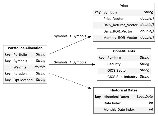
To begin, we create four placeholder tables where we will load our data:

• The portfolio allocation table containing instruments and weights per each optimization,
• The price table containing daily pricing data and rate of return information,
• A stocks table containing details around instruments attributes like GICS sector,
• And a dates table with the historical dates.

We use the portfolio table as our base table.

When joining tables, we can either explicitly set our mapping, or, if the tables share columns of the same name, Atoti will automatically join via those shared columns. When creating our cube, we use the default creation mode. In that mode, the non-numerical columns and the key columns are used for the list of hierarchies, while every numerical column will have corresponding sum and mean measures created.

Once our tables are created, we can load our data in. While in this example our data is stored in CSVs, we could just as easily load from data frames or other data formats. We can even set up a file watcher for automatic, real time updates.

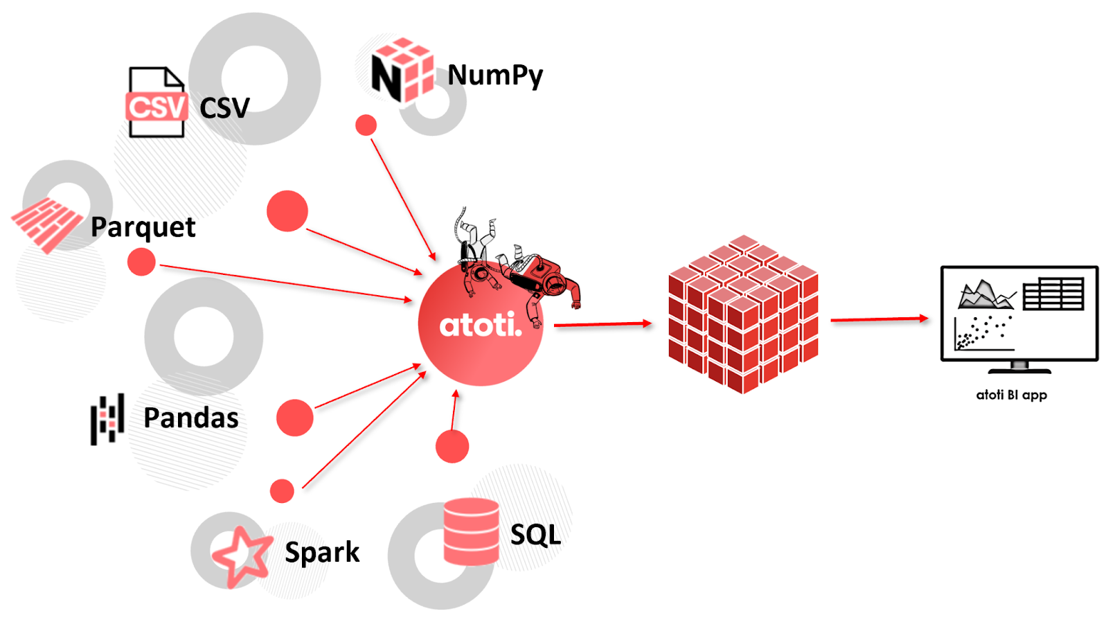
Through Atoti and its JupyterLab extension, we can immediately visualize and explore our data.

Metrics Definition

We compute a variety of important measures based on our array data to understand our potential portfolios’ performances. These include VaR, CVaR, Sharpe Ratio, and Error Tracking.

To complete these measures, we’ll first read in our array data from the underlying tables we loaded into.

m["Daily_Returns_Vector"] = tt.agg.single_value(price_tbl["Daily_Returns_Vector"])
m["Daily_ROR_Vector"] = tt.agg.single_value(price_tbl["Daily_ROR_Vector"])
m["Monthly_ROR_Vector"] = tt.agg.single_value(price_tbl["Monthly_ROR_Vector"])
m["Price_Vector"] = tt.agg.single_value(price_tbl["Price_Vector"])

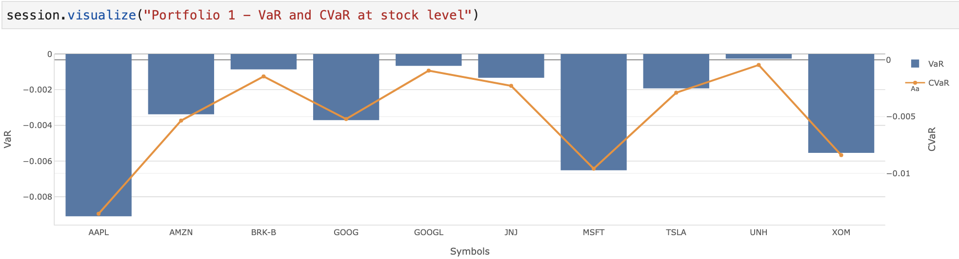
VaR and CVaR

Using our historical data and the newly created measures, we compute the Value at Risk and Conditional Value at Risk. Value at Risk is a statistical measure outlining the maximum loss of a portfolio at a given confidence level. Conditional Value at Risk, on the other hand, is the expected shortfall. It is given by the average of the losses on the remaining tail.

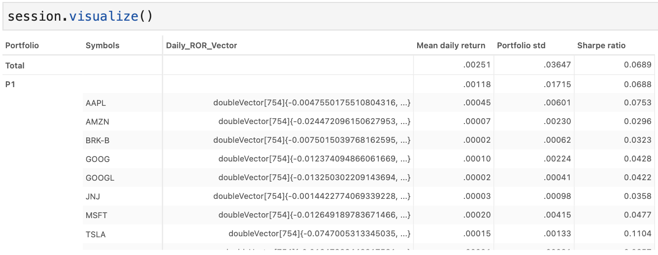
Sharpe Ratio

To measure the performance, we also compute the Sharpe Ratio:

Sharpe Ratio=(R_p−R_f)/σ_p

where R_p=Return of portfolio, R_f=Risk−free rate and σ_p=Standard deviation of the portfolio′s excess return (Volatility). The Sharpe Ratio measures the excess return of a portfolio, indicative of volatility. A larger Sharpe ratio indicates a risk-adjusted performance.

We assume a risk-free rate is 0% in our example.

Error Tracking

Also, using the initial portfolio as a benchmark, we compute the Tracking Error.

Tracking Error=σ(P−B)

where P = Daily Portfolio returns, B = Daily Portfolio returns of benchmark.

Portfolio Optimizer Integration

Now that we have our data loaded and our relevant metrics set up, we are ready to begin our optimization. In this example, we opted to use a pre-built optimizer, the Python API PyPortfolioOpt. As a reminder, the output of this library is a series of potential portfolios, constructed:

• for maximal Sharpe Ratio (max_sharpe),
• for nonconvex objectives (nonconvex),
• for hierarchical risk parity (HRPOpt),
• using Critical Line Algorithm (CLA),
• or to achieve minimum volatility (min_volatility).

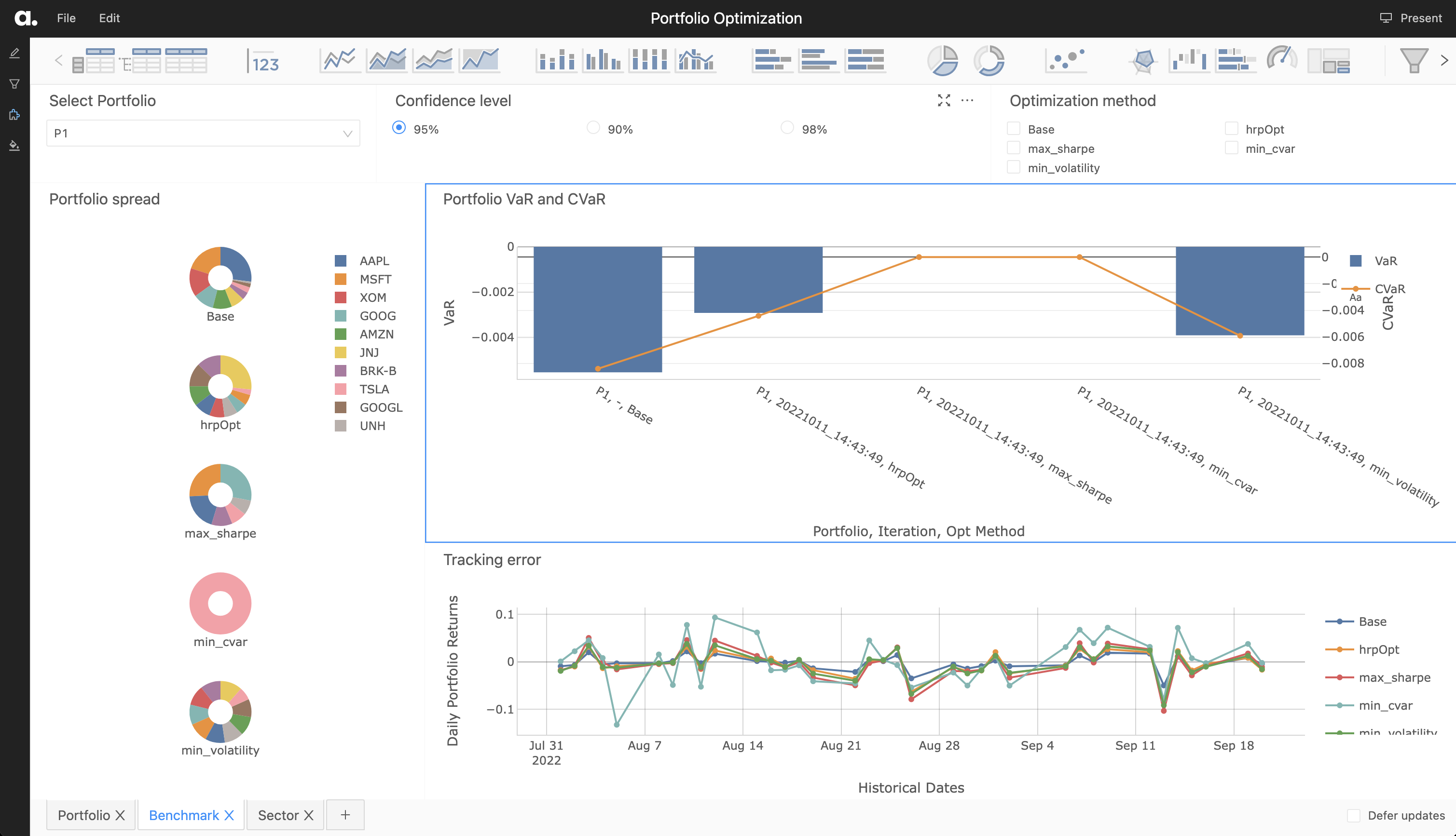
If exploring our notebook from our notebook gallery, the notebook uses iPyWidget to provide a button where a user can select a portfolio from the loaded portfolio table.

Our notebook also includes an option to explore the implementation using Atoti+ to customize the UI experience. Instead of using iPyWidget to provide a button for portfolio selection, the user can select portfolios from the dashboard. Readers with an existing Atoti+ license can directly view the implementation by switching the atoti_plus_license variable. Otherwise, reach out to ActiveViam for an Atoti+ license.

Once selected, the existing portfolio is sent to the optimizer, which runs and outputs weights per each optimization method as a dataframe. This dataframe of weights is then utilized to enrich the existing portfolio table with the newly constructed portfolios, with the Opt Method column containing the optimization method as specified in parenthesis in the above bulleted list.

Since the metrics have already been defined, we immediately can see the VaR, CVaR for each newly constructed portfolio. In fact, we can continue to iteratively pass portfolios through the optimizer and continue to compare across each portfolio returned, finding the portfolio which matches our desired Sharpe Ratio, CVaR, and tracking error.

Conclusion

This concludes our first part in our Portfolio optimization series, demonstrating how to connect an external or existing optimizer with Atoti to derive insights on how to adjust or optimize a portfolio. Stay tuned as we explore how we add constraints to the optimization, leveraging convex optimization theory.

To learn more, check out the corresponding notebook in our notebook gallery. Or reach out to ActiveViam to see how we integrate the CVaR optimization program into the BI analytics platform using Atoti+!