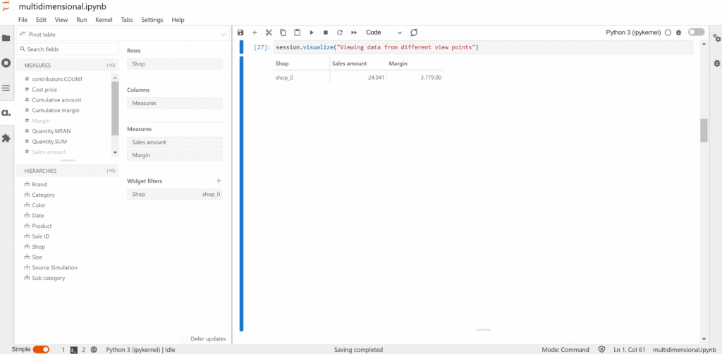
Multidimensional analysis gives the ability to view data from different viewpoints.

This is especially critical for business.

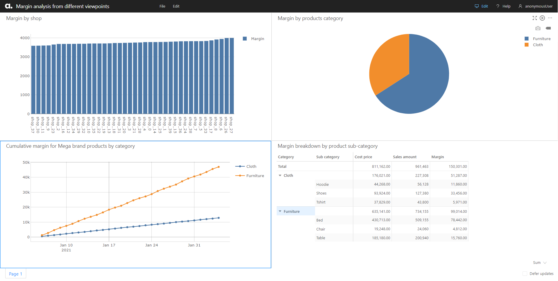
Let’s take a quick look at the few visualizations below.

We saw that with the same set of data, we are able to view the margin per shop, per product category, or for a specific brand or product, their margin getting broken down further by their subcategories. This difference in perspective can help businesses gather different insights.

What goes behind the scene?

To achieve these visualizations with relational databases, we will need a few kinds of SQL operations. Typically, there will be table joins, WHERE conditions to filter the data that we want and groupings by the different categories.

SELECT Sales.Shop, Sum(Sales.Quantity * Sales.UnitPrice) AS SalesAmount 
FROM Sales
LEFT JOIN Products ON Sales.Product = Products.Product
GROUP BY Sales.Shop;

With a multidimensional data cube, we have something equivalent to SQL as well. It’s called Multidimensional Expressions (MDX):

SELECT
  NON EMPTY {
      [Sales].[Shop].[Shop]
  } ON ROWS,
  NON EMPTY {
    [Measures].[Sales amount]
  } ON COLUMNS
  FROM [sales cube]

Unlike SQL, we don’t have to handle the “group by” with MDX and we are querying data that is pre-joined and aggregated. With a different semantic model and tools such as Excel or Atoti, users can query the cube without having to understand the complexities of the underlying data structures.

Now, the dashboard is a simple example of what multidimensional analysis offers. It gives us the ability to view data from the perspective of the shop, the products, the brands or anything else the business demands. Let’s see how this works with an OLAP cube.

What is OLAP?

You may have heard of OLAP, which is online analytical processing, or more recently, ROLAP (Relational OLAP), MOLAP (Multidimensional online analytical processing), HOLAP (Hybrid OLAP of the previous 2 approaches) and some other types. 

The current trend is in-memory OLAP, which loads the analytical data into memory for faster online calculations and querying. Basically, these are approaches to answer multi-dimensional analytical queries

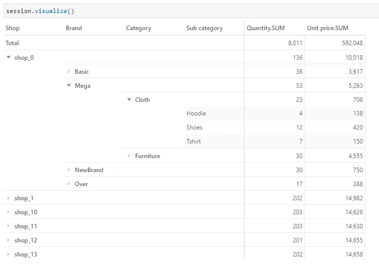
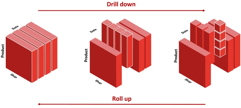
Two words commonly associated with multidimensional analysis are slice and dice.

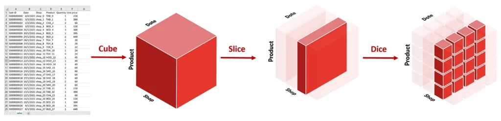
When we talk about slicing, we look at a particular group. For instance, if we would like to know about the product sales for a shop.

We can view the total sales of the shop. Or we can dice it by the Date and the Product to see the sales for each product on a daily basis.

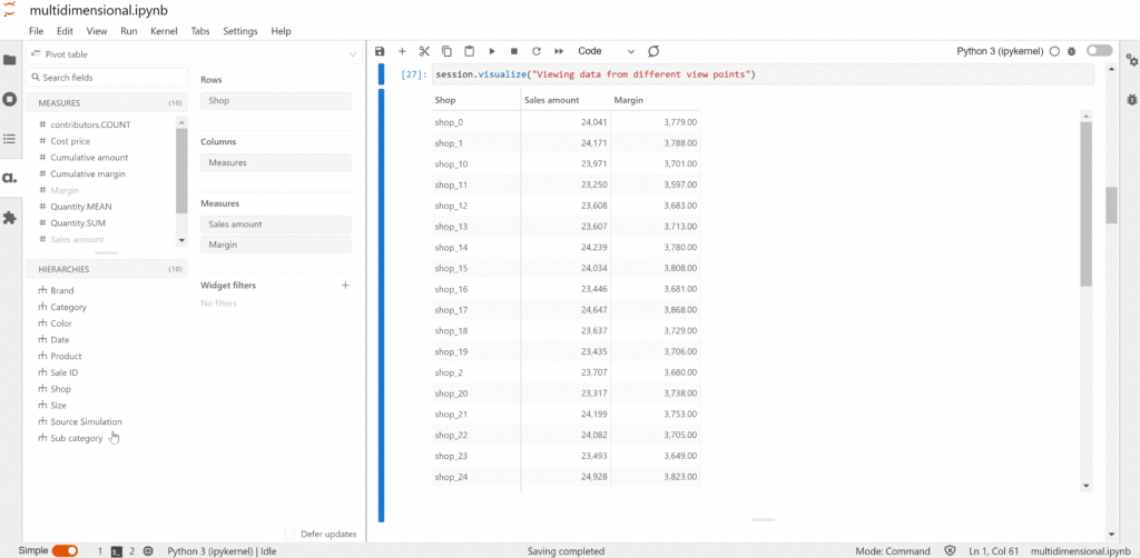
We can create a multidimensional data cube with the python library Atoti to help us understand the topic better. The full notebook can be accessed from the Atoti Github repository.

We can create a cube as follows:

import Atoti as tt
session = tt.create_session()

sales = session.read_csv("data/sales.csv")
cube = session.create_cube(sales, "sales cube")

When we look at the dataset, we see two categories of data:

• Numerical
• Non-numerical

Normally, numerical columns provide the measurements that businesses would like to know and we call them measures in a cube. But these numbers only make sense when we have the non-numerical descriptions that tell us what these values are. Thus, the non-numerical columns, also known as dimensions, comes into the picture and each value of the dimension is called a member.

How do we handle multiple data sources with a cube?

It is common that we join tables in databases to get a combined view. The same thing applies to a cube. We can have multiple tables joined together.

products = session.read_csv("data/products.csv", keys=["Product"])
sales.join(products)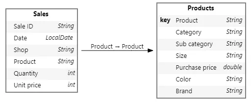

Once we have that, we can slice and dice across the dimensions of all the tables in the cube once they are joined. In this particular case, you can see that I have joined the new table called products and it has information such as the brand and category.

What can we do with dimensions and measures?

Let’s explore a little about the attributes of a cube.

We have the dimensions such as Products and Sales that groups the hierarchies and the hierarchies group the levels.

For instance, instead of having Categories and Subcategories as two separate hierarchies, we can merge both as levels under the same hierarchy. We’ll be able to expand on them in our pivot table without having to add them individually.

With this semantic model, how data is being joined is obscured from users. They can simply select the hierarchies and measurements that they need for their analysis.

Preprocessing or post-processing 

One last important concept: let’s look at when to perform preprocessing and when to perform post-processing. 

Preprocessing – trading storage consumption for computational efficiency

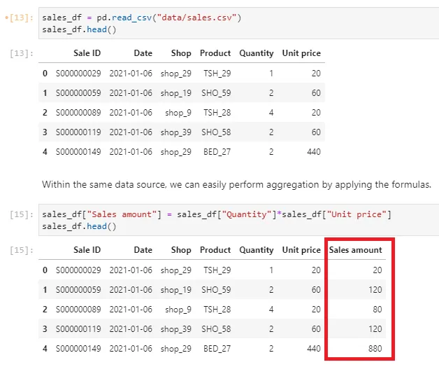
We spoke of measures earlier on as numerical columns from the incoming data source. These could be granular measurements such as quantity and unit price. From this, we could compute the sales amount, simply by multiplying quantity with the unit price. We can do so with Pandas below:

import pandas as pd

sales_df = pd.read_csv("data/sales.csv")
sales_df["Sales amount"] = sales_df["Quantity"]*sales_df["Unit price"]

As a result, our dataset is now bigger, with an additional column.

In this case, we have just traded the storage consumption for computational efficiency because the cube is not required to compute the sales amount on the fly.

And this is only possible if we are pre-processing the measure at the most granular level – per sales. Consequently, we will be able to drill down (giving the most granular value) or roll up (giving the aggregated value) for this measure.

This cannot be done for the other levels of data granularity such as the sub-total or grand total level. It’s because there is no means of knowing how to break it down as we drill down on the different hierarchies.

One example of this is the cumulative margin. Imagine the effort we need to put in, to pre-compute the cumulative margin per store or per product each time the management wants a different perspective. It’s just not viable to pre-compute.

So, this is where post-processing in the cube helps – we compute what we need on the fly.

Post-processing – computes on the fly and provides flexibility

Let’s imagine a scenario where one of the shops was late in submitting their sales for a particular day. With pre-processing, we will have to recalculate everything and probably reload a lot of data.

However, we can simply upload the missing data with post-processing. The measures that we have defined earlier will take care of the computation for us.

As we can see in the GIF above, the data on 15th Jan where the margin and cumulative margin increase as we load the missing sales of shop_0.

Hopefully, this article gives you a good peek into multidimensional analysis.  For examples of multidimensional analysis in action, visit the Atoti notebook gallery or read our Retail Pricing Case Study.