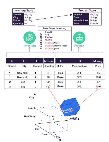
In Atoti, we integrate data from different sources into an in-memory data cube. Without worrying about the data semantic layer, users are able to query along different hierarchies to gain insight from different perspectives.

In this article, we will take a look at the different types of querying that can be performed in Atoti, their output and constraints.

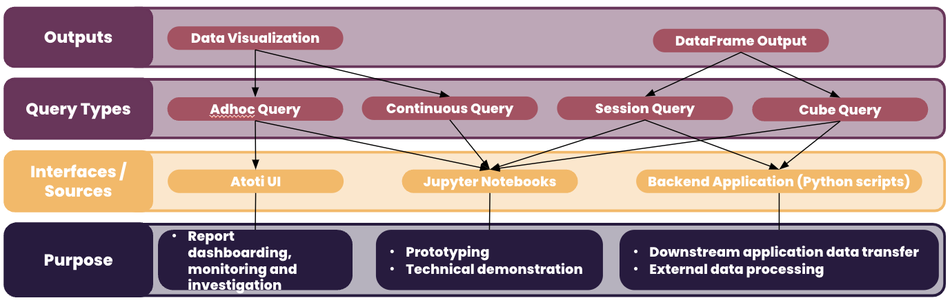
Types of query

Let’s view querying from the desired output perspective.

Data Visualization

Data visualization helps to enhance understanding of complex data through summarized values displayed over pivot tables or charts. 

Ad-hoc Querying

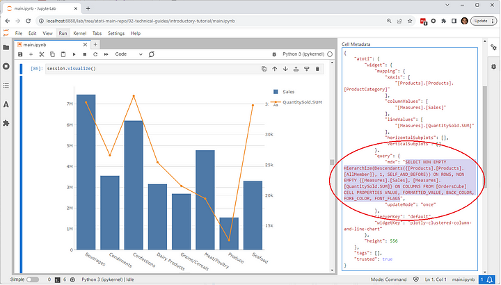
Atoti allows users to interactively build their own visualizations without having to worry about the syntax for the query. In fact, the Multidimensional Expressions (MDX) query is formulated by the application as we build our visualizations.

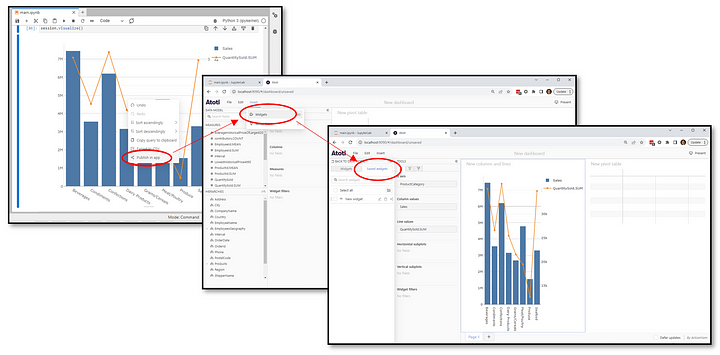
Visualizations are in fact widgets that can be used in both Jupyter Notebooks and the Atoti UI. We can export them from the notebook into the Atoti UI.

Such queries are ad-hoc as the data is retrieved at the point of querying when the cell is executed or widgets get loaded in a dashboard. There is no further querying from the widget unless a refresh is triggered.

Continuous Querying

One difference between the visualizations in Jupyter Notebooks and on Atoti UI is the ability to support continuous querying.

Continuous queries are “normal” Atoti queries, but instead of just making a query and getting the result at a given instant, they are refreshed when data changes.

Continuous queries are registered in Atoti Server together with their listeners. When the values of the measures defined in the registered query change because of a transaction or a real-time event, the listeners are notified of this change and receive the new aggregated values.

To turn on continuous querying on the Atoti UI, simply go to the intended widget and toggle the following icon:

Continuous querying is only made possible because Atoti supports incremental data loading. This means that we can load data into the cube at any time without having to restart the entire application.

Check out the notebook Real-time aggregation with Atoti to try out continuous querying.

Tips for working with widgets

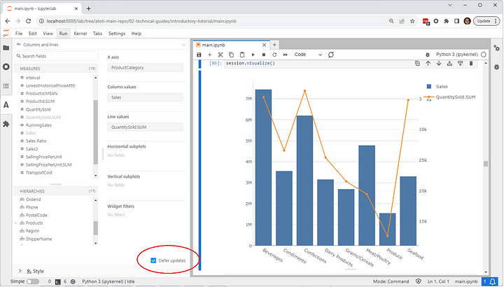
💡For all widgets, we can delay the querying with the “Defer updates” checkbox until we are done adding in the levels and measures that we needed.  

💡With Atoti tables, data is loaded with a lazy loading mechanism. 

Only a portion of data corresponding within the visible area of the table is initially loaded into the client. New chunks of data are loaded as the user scrolls. 

💡For charts loading large amounts of data, it may take a while to render. In case you need a longer time for the query to return, we can increase the limit within the widget when the querying stops on timeout.

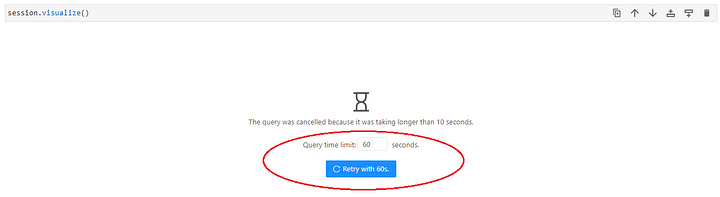
Alternatively, we can programmatically set a longer timeout period for the widgets generally using the cube.shared_context. The default timeout is 30 seconds.

cube = session.create_cube(table)
cube.shared_context["queriesTimeLimit"] = 60

DataFrame Output

Sometimes, we may want to output data from the cube for further processing such as:

• Passing to a downstream system such as risk engines or machine learning applications
• Modification for simulations

To do so, we can programmatically query the cube using either:

• Cube query which uses Atoti syntax to query a specific cube
• Session query which uses MDX for querying

Cube Querying

Without having hard to craft MDX, we can easily query the cube by defining the measures on the levels we require. We can select a subset of the data by applying filters. However, note that the filter can only work on level equality with a string.

Since it is a cube query, it retrieves data only from the specific cube variable we work with:

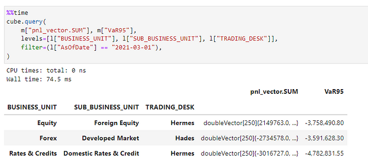
cube.query(
    m["pnl_vector.SUM"], m["VaR95"],
    levels=[l["BUSINESS_UNIT"], l["SUB_BUSINESS_UNIT"], l["TRADING_DESK"]],
    filter=(l["AsOfDate"] == "2021-03-01"),
)

We can list as many measures as required, separated by commas. Define the levels in a list.

Tips for Cube Query

💡The query result returns in a DataFrame in “pretty” mode by default. This means the levels queried are the indices to the measures and the dataset is sorted by level order:

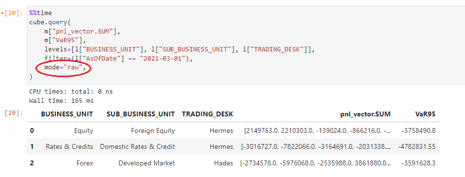
We can also set the mode to “raw” for large exports which is faster and more efficient:

💡For large query sets, we can increase the timeout period with the timeout parameter. It is defaulted to 30 seconds, similar to the widgets. 

import datetime
cube.query(
    m["SimulatedRate"],
    levels=[l["HistoricalDate"], l["RiskFactor"]],
    timeout=datetime.timedelta(seconds=120),
)

Session Querying

It may take a little effort to craft an MDX, session querying however, provides greater flexibility than cube querying. For instance, while we are unable to filter by range with cube query, we can formulate our MDX to do so:

session.query_mdx(
    """
     SELECT
      NON EMPTY {
        [Measures].[contributors.COUNT],
        [Measures].[Price],
        [Measures].[Vol],
        [Measures].[Rate]
      } ON COLUMNS,
      NON EMPTY Crossjoin(
          [Underlyings].[Underlying Id].[Underlying Id],
          LastPeriods(250, [Market Data].[Trans Date].[Trans Date].[2023-10-01])
      )
      ON ROWS
     FROM [TRANSACTIONS]
    """
)

Using the MDX function LastPeriods, we are able to retrieve the measures Price, Vol and Rate for the last 250 members from 2023-10-01. Note that in this case, we are retrieving past 250 available dates before 2023-10-01 and the dates between 24-01-2023 to 2023-10-01.

Also, using the session query, we are able to select from any cubes within the session depending on the MDX formulated.

💡Similar to cube query, we have the same “mode” and “timeout” parameters. 

Purpose of query

With most front-end users, we would choose to work with the visualizations which are easier to understand. Front-end users can export the underlying data from the visualizations into CSV: 

However, for large data extraction or batch processing, use session or cube querying instead. From the DataFrame, we can export the data to the necessary output type.

So, now we know the types of querying options we have, it’s time to give Atoti a try!